Authors: Shahrzad Azizzadeh, Kaustubh Khandwe, Bahar Biller, and Paul Venditti
On large-scale solar farms, power loss is the silent drain on profits. Unoptimized panels chip away at efficiency, causing hidden losses that people often overlook—but those losses are never insignificant. In this post, we’ll uncover how to spot and solve these inefficiencies. Drawing from a real-world U.S. case study, you’ll see how SAS machine learning algorithms turn vague estimates into accurate forecasts of power loss in solar farms. The result? A clear, data-driven roadmap for smarter operational decisions, improved system efficiency, and ultimately, stronger profitability.
Background
In the rapidly growing field of renewable energy, solar farms play a vital role in supplying clean electricity to the grid. Yet, even with advances in technology, installations can underperform due to subtle and often invisible issues. This includes issues such as misaligned panels, weather-related impacts, or gradual wear and tear. These inefficiencies are not always apparent in daily operations. They can accumulate over time, resulting in significant revenue loss and reduced energy output.
To put this in perspective, panel angle deviations from optimal positioning can reduce power output by 2-8%. Panel degradation typically causes 0.5-0.8% power loss annually, accumulating to 15-20% over a panel's 25-year lifespan. Perhaps most significantly, high surface temperatures during peak operating hours can cause temporary power losses of 10-20% when panels reach 60-70°C. This represents millions of dollars in lost revenue for utility-scale installations. This is why the ability to anticipate and quantify those losses is so important, especially at scale.
Multiple factors contribute to performance degradation, including suboptimal panel tilt angles, adverse conditions, and equipment aging. By using historical data and advanced modeling techniques, we demonstrate how SAS machine learning procedures can be employed to construct a predictive framework that quantifies power loss in relation to ideal operating conditions. This model enables operators to isolate inefficiencies, forecast degradation trends, and proactively manage maintenance.
The resulting insights are essential not only for maximizing energy yield but also for supporting financial planning and grid reliability. We will outline the end-to-end analytical process, including data preprocessing, predictor variable selection, model development, and validation. We also include visualizations by using the SGPLOT and GCHART procedures that highlight key insights and inverter-level performance findings.
Use case
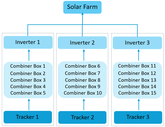
Figure 1 illustrates an asset hierarchy in a solar farm with three inverters. Each is connected to a set of combiner boxes, which in turn are connected to a collection of solar panels. Each sub-system, consisting of an inverter, a set of combiner boxes, and a collection of solar panels, includes a solar tracker system. This is responsible for adjusting panel tilts. All panels connected to a combiner box share the same design and orientation. They, therefore, share the same optimal angle for maximum sun exposure. Several sensors monitor various environmental and operational variables at five-minute intervals.
Guided by discussions with industry experts, we established a set of assumptions to support the prediction of power loss in the solar energy system. Losses are evaluated at both the inverter and combiner box levels. The example system in this post consists of 15 combiner boxes. they are organized into three groups that supply direct current (DC) power to three solar inverters. Each combiner box connects to a set of identical solar panels, ensuring uniform performance characteristics.
For modeling purposes, we assume that the sun delivers consistent solar irradiance—defined as power per unit area—across all panels connected to the same combiner box. Although this assumption simplifies the modeling process, it does not fully reflect real-world conditions. Factors such as shading, dust accumulation, or panel soiling can cause non-uniform irradiance, which can impact performance. These conditions can limit model accuracy, as a result. Future work could explore the incorporation of spatial variability into irradiance measurements.
Input data
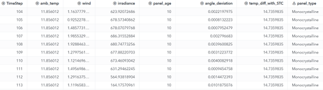
A snapshot of 10 sample rows from the analytics base table, used as the input data set for our project, is shown in Figure 2. In this table, the TimeStep column represents the timestamp at 5-minute intervals. amb_temp indicates the ambient air temperature at the site, measured in degrees Celsius at the time of the reading. wind refers to the wind speed at the solar farm, recorded in meters per second (m/s). irradiance refers to the solar irradiance on the panel surface, measured in watts per square meter (W/m²).
Panel_age denotes the age of the photovoltaic (PV) panel in years since installation. angle_deviation measures the difference between the panel’s actual tilt and its optimal orientation, in radians. temp_diff_with_STC represents the deviation of the panel surface temperature from the Standard Test Condition (25 °C), also in degrees Celsius. Finally, panel_type specifies the material used in the solar module. The objective is to understand how these factors affect the power loss experienced by each inverter shown in Figure 1.
Model
Based on data availability and the primary factors contributing to power loss, we focused our analysis on three key categories:
- Performance degradation due to equipment aging
- Sub-optimal panel tilt angles
- Temperature-related losses caused by device overheating and thermal fluctuations.
The historical data set does not directly include power loss values. However, it contains several operational variables that influence and contribute to power loss. Table 1 summarizes the methods used to compute power loss for each of the three identified categories. In this content, Pcurrent refers to the actual direct output power generated. Ploss represents the estimated power loss.
| Category | Loss Calculation Method |
| Equipment Aging | Linear degradation model (Jordan, Dirk C., and Sarah R. Kurtz) based on panel age (in years), with degradation rates varying by panel material: Ploss = Pcurrent x \(\frac{degradation\_rate\; x\; average \;panel \;age} {1\; -\; degradation\_rate \;x \;average \;panel \;age}\) |
| Panel Angle Deviation | The amount of loss (Barbón, J., Fernández-Ibáñez, E., and Martínez-Alonso, M) is affected by the cosine of the difference between the optimal and current angles: Ploss = \(\frac{P_{current}} {cos(angle\_deviation)}\) - Pcurrent |
| Temperature Effects | A coefficient is applied (Dash, P. K., and N. C. Gupta) to represent the fractional power loss per °C increase above the Standard Testing Condition (STC) temperature of 25°C: Ploss = Pcurrent x \(\frac{\gamma\Delta\tau} {1\;-\;\gamma\Delta\tau\:}\) |
Table 1: Power loss calculation method
The target variable for the predictive model is Pcurrent, which represents the actual power output. Once this value is predicted, power loss (Ploss) is calculated for each observation using the methods outlined in Table 1. The model uses temperature, wind speed, and solar irradiance as predictor variables. The model excludes factors like panel age, angle deviation, and temperature deviation from standard test conditions as predictors and applies them after prediction to calculate power loss. Because the original data set was recorded at 5-minute intervals, it was aggregated to hourly intervals to improve the clarity of insights and visualizations related to power loss.
We split the data into training and testing sets using a 70:30 ratio. Power output predictions were generated by using the FOREST and GRADBOOST procedures, with the model achieving the lowest Average Squared Error (ASE) on the test set selected for final deployment. To enhance interpretability, in addition to the variable importance scores, Shapley values were calculated using the TreeSHAP option in the ASTORE procedure. We shared the results through both data sets and visualizations.
Results
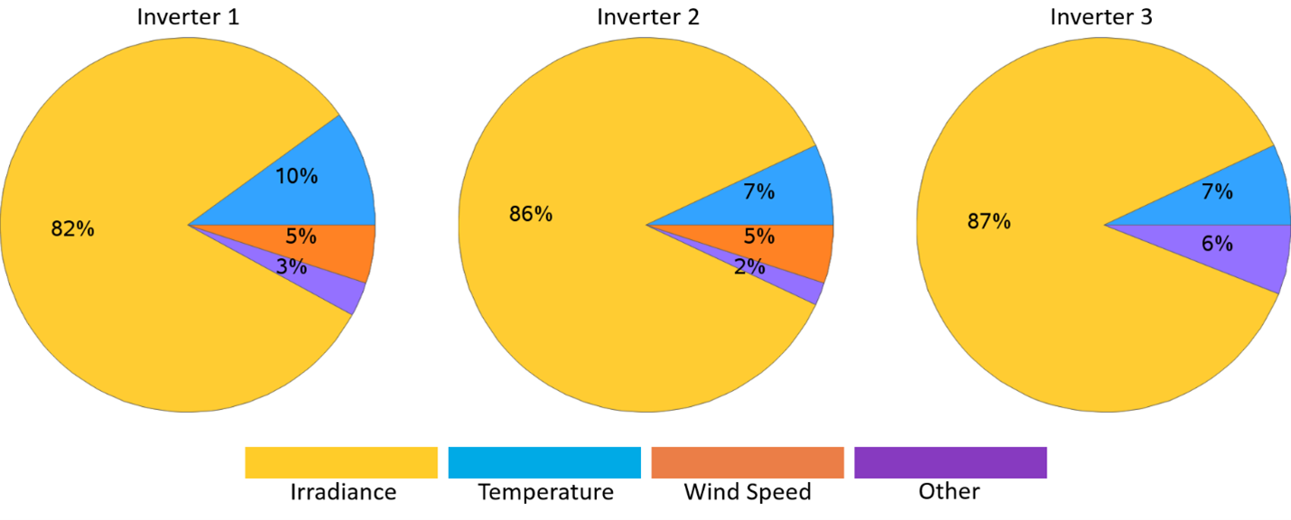
Figure 3 illustrates the relative importance of each predictor variable for the target variable Pcurrent. This represents the sum of the direct currents emanating from all the combiner boxes connected to each inverter. We quickly identify irradiance as the primary variable affecting power generation, followed by ambient temperature and wind speed.
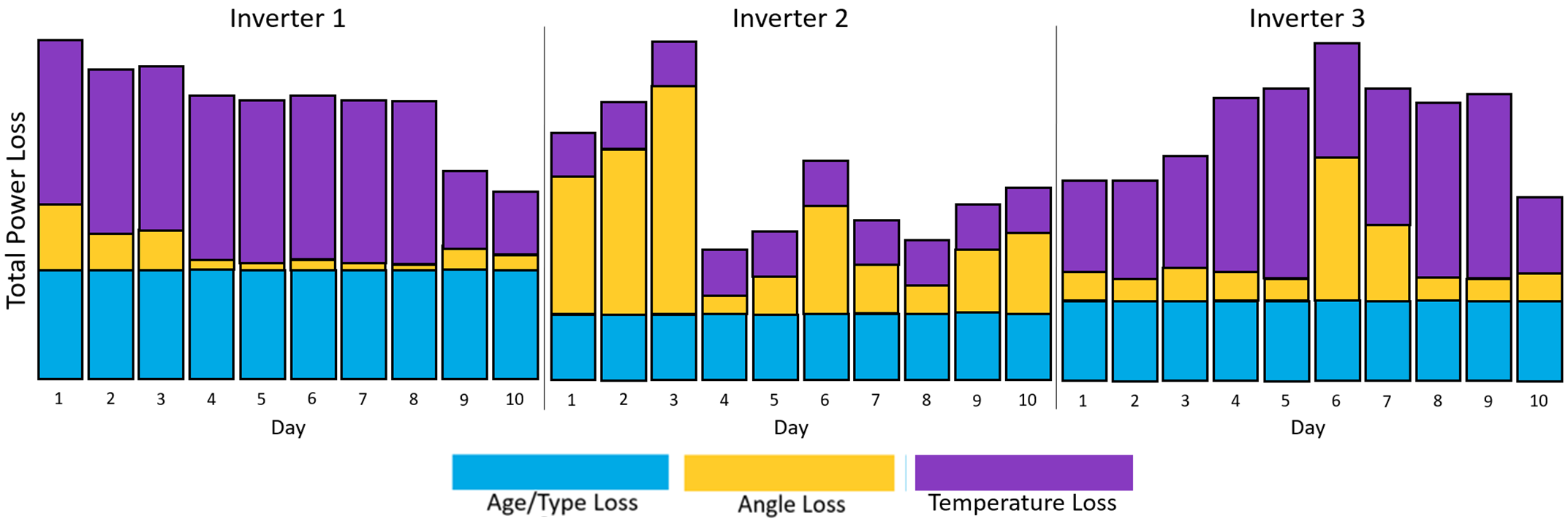
On the other hand, Figure 4 illustrates the power loss by category for each inverter over a 10-day period. For Inverter 1, the percentage of power loss due to panel angle deviation is small, indicating the tracker system is working as expected. For Inverter 2, however, the tracker system appears to be experiencing issues during the first three days. Temperature-related power loss plays a major role for inverters 1 and 3, indicating the overheating of the panels, and the need to monitor the cooling systems.
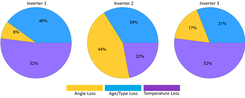
Finally, the pie charts of Figure 5 summarize the share of each power loss over the same 10-day period, for each inverter system.
Conclusion
This post presents a practical, end-to-end framework for forecasting power loss in utility-scale solar farms using SAS Viya. By integrating domain expertise, such as panel degradation behavior, tilt misalignment effects, and temperature sensitivity, with advanced machine learning methods, we achieved a comprehensive understanding of power loss dynamics. Our approach enabled us to quantify power loss drivers at both the inverter and combiner‐box levels, forecast actual power output, and translate those predictions into interpretable, category-specific loss estimates. By using Shapley-value analysis, we also identified the environmental and operational variables that have the most significant impact on performance deviations.
Insights from our case study revealed that temperature fluctuations were the leading cause of power loss in two of the three inverters. Solar tracking systems generally maintain optimal alignment. These findings empower operators to prioritize cooling system maintenance, optimize tracker calibration, and schedule targeted inspections. This ultimately enhanced energy yield and minimized downtime. The economic impact of these insights cannot be overstated: with individual loss factors capable of reducing power output by 2-20% depending on the issue, our predictive framework addresses inefficiencies that could otherwise cost utility-scale solar farms millions of dollars annually in lost energy production. By combining predictive accuracy with interpretability, this framework lays a strong foundation for proactive, data-driven solar asset management.
Paul Venditti
Paul Venditti is a seasoned industry consultant with over three decades of experience in industrial analytics and digital transformation. His career began in heavy equipment services and extended through a decade at GE Research, where he patented advanced analytics and digital twin solutions. At SAS, as an Advisory Industry Consultant, Paul helps organizations leverage AI, IoT, and machine learning to enhance manufacturing quality, minimize downtime, and drive operational resilience.
Kaustubh Khandwe
Kaustubh Khandwe is a Senior Data Scientist in the SAS Pune Applied AI and Modeling (AAIM) Division. He has developed solutions across various industries, including manufacturing, retail, and IOT. With AAIM, he has contributed to projects such as Preventive Maintenance for Solar and Wind Farms and Auto Damage Fraud Detection in the Insurance industry. Future goals include building industry-impactful models and driving their integration with cutting-edge technologies, such as Agentic AI, ultimately providing a value-driven software experience to customers.